Model card: variability index

What it is

Overview

Addressing field heterogeneity is a major opportunity for yield and productivity optimization by enabling growers to adapt resource utilization at a sub-field level so as to increase the profitability of any farm inputs.

This model provides several field indexes that enable assessment and comparison of field heterogeneity. These insights allow to fine-tune agronomical recommendations, such as the profitability of adopting variable rate techniques, and to order fields by their variability level.

The indexes calculated by this algorithm can be used to understand the heterogeneity and consistency of a given field. This information can leverage different agronomic discussions and decisions, such as understanding the potential of using variable seed density or variable product and fertilizer rates techniques on a specific field. The API outputs are Consistency Index (consistency), Variability Index (variability), and Variability x Consistency (vxc).

Inputs

• The Cropwise field_id associated with specific field boundaries as captured in Cropwise Farm settings
• start_date and end_date of the historical period within which satellite images should be fetched for computing the indexes

Default values: If not provided the default interval will be of five years, starting from the previous day and going back five full years.

• start_date: today - 5 years
• end_date: today - 1 day

Outputs

The model returns 3 values and a list of season information used to calculate those indexes.

1. Variability index (variability):

• Answers the question 'Considering multiple crop seasons: How variable is the vegetation in the field?'.
• Low values indicate homogeneous vegetation growth in the field, whereas high values indicate contrast in growth among different areas.

2. Consistency Index (consistency):

• Answers the question 'Is the crop spatial heterogeneity consistent over multiple seasons or not?'
• Low values indicate an erratic spatial structure, whereas high values indicate consistent spatial structure across seasons.

3. VxC index (vxc):

• Weighted average between VI and CI = (VI ×0.67) + (CI ×0.33).
• This value gives an overall assessment of how variable and how consistent the spatial structure of vegetation is in a field.

4. Seasons:

• Array of the selected seasons, with their start_date, end_date, peak_date, and season (summer, spring, autumn, or winter).

API Endpoint structure

These indexes are currently available in the variability_index endpoint or as a sub-model within the productivity_zones API.

How to use

Satellite subscription

The desired field has to be registered in Cropwise under an organization subscribed to a valid license to use Cropwise Satellite Image Service.

Area of validity

The algorithm is capable of calculating the indexes for extensive annual field crops (corn, wheat, soybeans, etc.). It's independent of the country.

Limitations

• Extremely cloudy areas may lack sufficient images, which may decrease the quality of the final result.
• The model uses Sentinel 2 images with 10x10 m pixels. Hence it is not recommended to use the model for fields below 1 ha.

Default Configuration

By default, the output is a dictionary with 3 indexes (variability, consistency, and vxc) and the seasons used for their calculation.

By default, the model uses all available crop seasons specified in the parameters to calculate the indexes. Each crop season represents a single crop, not a calendar year, so fields with double cropping will show two seasons for the same year.

If any season is split between multiple crops, the algorithm automatically excludes those seasons from the analysis. This prevents skewed results in the final productivity zoning. If all identified seasons for a field are split between different crops, there will not be enough data to run the model, and an error message will be returned.

Custom Configuration

Users can edit the start_date and end_date to change the historical period used to calculate the indexes.

How to interpret insights

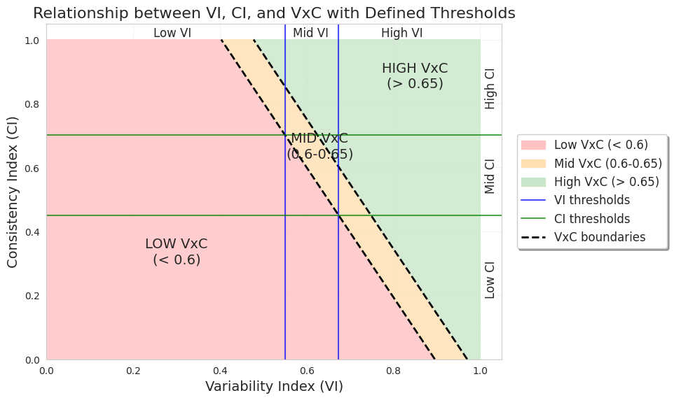
The relationship between these metrics guides management recommendations:

• Low variability + Low consistency suggests limited benefits from variable rate applications
• High variability + Low consistency indicates seasonal or management factors may be influencing patterns, requiring further investigation
• High variability + High consistency presents the best opportunity for precision agriculture, with stable zones that can be reliably managed differently
• Low variability + High consistency may still benefit from targeted applications despite subtle differences

Higher vxc scores generally indicate greater potential for optimizing inputs and yields through precision agriculture techniques.

variability_thresholds = [0.55, 0.6738]  # Low < 0.55, 0.55 <= Mid <= 0.6738, High > 0.6738
consistency_thresholds = [0.45, 0.7015]  # Low < 0.45, 0.45 <= Mid <= 0.7015, High > 0.7015
vxc_thresholds = [0.60, 0.65]  # Low < 0.6, 0.6 <= Mid <= 0.65, High > 0.65

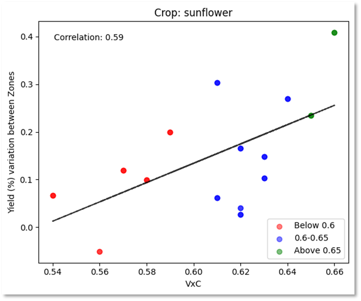
Use-case example

VRA Effectiveness Increases with VxC: Fields with higher vxc scores demonstrate greater yield differences between management zones, directly translating to larger potential benefits from variable rate applications of seeds and fertilizers.

Economic Justification: The yield variation range (0-40%) suggests that high vxc fields could see substantial economic returns from precision agriculture, while low vxc fields may not justify the additional input costs and complexity.

Field Selection Strategy: This relationship supports using vxc scores as a screening tool - prioritize precision agriculture investments in fields with vxc>0.65, investigate moderate potential fields (0.6-0.65) with additional data, and maintain uniform management in low vxc fields.

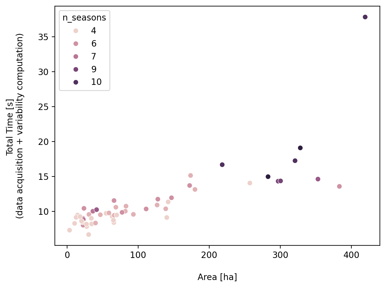
System information

Dealing with a historical set of images can be time-consuming, with processing times proportional to field size. On average, for fields of ~200ha, response times can reach up to 25 seconds. For larger fields or during periods of high load, processing times are expected to increase further.

It's recommended to maintain a rate of 1 request per 3 seconds for fields under 100ha and 1 request per 10 seconds for fields larger than 100ha. A more systematic breakdown of processing time versus field size can be seen in the plot below.

Last update: 06/10/2025 JLP